Rapidly rising inflation, bear markets, Congressional hearings over political misdeeds, geopolitically related energy price spikes. What next? Bell-bottom pants? The return of disco? These are not echoes of the 70s that people might have hoped for.

We are living in a time with many similarities to that era, including concerns about how to protect one’s portfolio – with cash losing value to inflation and the stock market suffering the worst six-month start of a year since 1970. There are also some differences. The unemployment rate is lower than during the stagflation of the 70s. On the other hand, at least on a nominal basis, bonds in the 70s paid a fair amount of interest unlike now.

All of this suggests that it would be instructive to look at the 70s to see how different strategies performed. While not a perfect match to today, the 70s can still offer some insights.

To address the fact that nominal rates are lower now and bonds are losing real value more quickly, a few of the allocation strategies here are comprised primarily of stocks and cash. If those low bond allocations fared relatively well in the 70s, that gives hope for low/no bond portfolios faring at least as well today.

Rationales for asset allocation

Over the long term, equities beat bonds, yet investors allocate their portfolios more conservatively. Part of the reason is psychological. Part is because risk becomes real when people need to spend down some of their assets.

If people were investing forever with no intention of withdrawing money, they might as well put everything into equities and walk away. That’s somewhat like saying that a rock is the fastest computer – you just can’t tell because it has no I/O.

For the exercise here, the investor is the prototypical retiree who starts withdrawing 4% of a portfolio and adjusts that amount annually for inflation.

 The “experiments”

To recap: we are going to try to simulate the worst-case experience for an investor in retirement. That pretty much summarizes our target window: a crushing equity bear, the end of a long bond bear market, market instability, and incessant price inflation. The question is, what strategy offers the most hope for a retirement investor.

I stipulate “retirement investor” because the interests of folks in the “decumulation” phase of their investing careers are very different from, and almost diametrically opposed to, the interests of investors just beginning. For our readers in their 20s and 30s, the thing you should pray for is a really dramatic decline in stock prices, which will reset the market and set you up for decades of robust returns as you build your portfolios. (And yes, the rest of us will be driving our Buicks slower than usual with our left turn blinkers on just to p*** you off.)

Ten years is a conventional period for looking at performance. The decade I used is 1973 – 1982. This period started with a crushing two-year bear market. That tests resilience to the sequence of return risk. The market had large swings in performance from year to year. That’s good for testing reallocation schemes. Rampant inflation began in 1973 and lasted through 1981. So the decade chosen here neatly coincides with the entire high inflation period.

Six different stock allocations are used, ranging from 40% to 100%.

• 40% stock – a traditional Wellesley-like allocation, with the rest in bonds.
• 55% declining to 40% – a target date glide path, numerically similar to those by Rowe Price.
• 60% stock – a traditional Wellington-like allocation, with the rest in bonds.
• 75% stock, 16% cash, 9% bond – reduced bond allocation, with cash for four years (4 x 4%)
• 90% stock – Warren Buffett proposed this in his 2013 shareholder letter; the rest in cash.
• 100% stock – for comparison

Each of these portfolios is rebalanced annually after the investor make a 4% withdrawal (adjusted for inflation). A second reallocation scheme is also tested with the two bond-light portfolios (75% and 90% stock).

The idea is to use the cash to “protect” against drawing from equities when they are down in value. This “cash buffer” approach is implemented by drawing against cash (then bonds, if any) so long as equities are below their high-water mark in dollars. Once equities recover and surpass their high-water mark, the excess is used to replenish the cash allocation (and bonds if any). Once the value of the entire portfolio exceeds its high-water mark, standard rebalancing resumes, i.e. 90/10 or 75/9/16.

This sounds like a bucket approach. It differs in that traditionally one always rebalances after drawing money from whichever bucket did the best. As Michael Kitces explained a few years ago, that approach is little different from simply using a balanced fund since you are always maintaining the same allocations. The “cash buffer” approach tried here is not the same.

The numbers

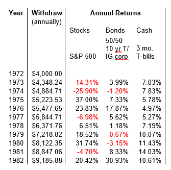
Source: Historical Returns on Stocks, Bonds, and Bills: 1928-2021

The investor starts with $100,000 at the end of 1972 and immediately withdraws 4%. The withdrawal amount is adjusted annually for inflation. For bond returns, a 50/50 mix of 10-year Treasuries and investment-grade corporates are used.

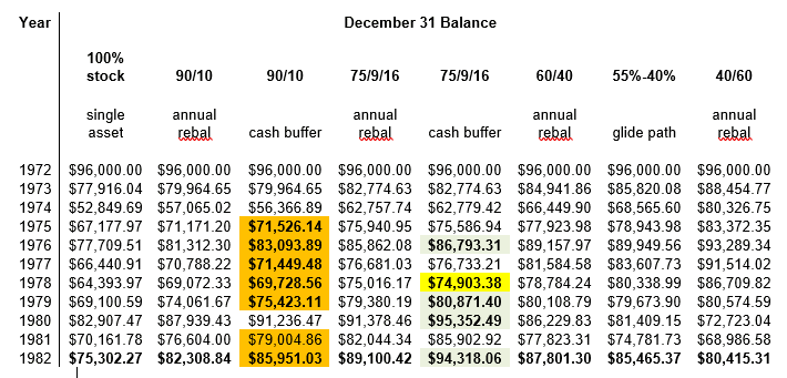
The year-end balances for each of the portfolios are shown in the table below. The highlighted cells are discussed in the next section.

Observations

1. Equity exposure matters, a lot. Invest too much in stock (above 75%) or too little in stock (below around the 50% mark) and performance declines. Too much stock and sequence of return risk severely hurts the performance. At the end of 1974 after two years of heavy stock losses, the pure equity portfolio was down to $53,000. It never recovered. With too little stock a portfolio falls behind in the good years. The 40/60 portfolio was leading at the end of 1977. But then equities came roaring back and it fell behind.

   If the stock market goes straight up, as it did between 2009 and 2021 (only in 2018 did it have a modest loss), then the more equity in the portfolio, the better the portfolio’s ending value. But one can’t count on a consistently rising market.

2. Cash counts. The cash buffer approach can make an appreciable improvement in performance. The 75% stock portfolio using the cash buffer approach ended with nearly as much as it started with. (Unfortunately, that is in nominal dollars; the dollar lost more than half its value over this decade.) The other portfolios did not come close.

   A bit of good news is that when these portfolios are run over the ten-year period ending May 31, 2022, the cash buffer approach still beats conventional rebalancing, at least for the two portfolios tested here. The margin isn’t much, but it inspires confidence that this may be a robust approach to eking out a little higher return.

3. A “cash stash” is critical. Too small a cash allocation with the cash buffer approach can leave one depleted of cash for years when the market is down. The orange cells in the 90/10 allocation represent years when there was no cash left and subsequent withdrawals were coming from equities. It is somewhat amazing that this approach still managed to outperform the annual rebalancing approach.

   The yellow cell in the 75/9/16 allocation represents the only year in which cash was depleted. Even then, there were still bonds available to protect against drawing from equity. But it was close. One more bad year and the bonds would have been depleted as well. At least based on the decade tested here, 75% equity is a propitious allocation.

4. A cash stash increases long-term returns. The cash buffer protection of equities in the 75% portfolio was adequate for equities to fully recover and to add value back to cash (and bonds). This happened in the years with the green (okay, “faint sage”) cells.

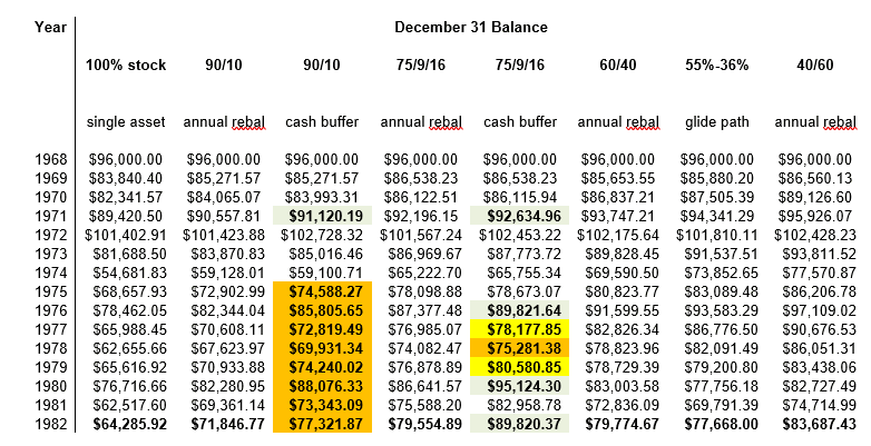
5. Where you look determines what you see. The ten-year annualized returns of an equity fund can change dramatically with a shift of as little as three months in the period you’re tracking. That’s one of the reasons that MFO warns against over-reliance on arbitrary comparison periods that are simply based on the number of fingers and toes you have. (Really. That’s why 5 / 10 / 20 is so common.) It’s more informative, we think, to look at performance across entire market cycles when we can: capturing both the bad times and the good times gives a better picture of your actual experience.

   That’s important here because our bottom-line numbers and strategy success rates change if you extend the analysis period by four years, starting with the bear market of 1968 rather than the bear market of 1972. Here’s what we would see then.

   

Conclusion

Shifting bonds to stocks and cash, thus increasing the allocations of each, has the potential to somewhat improve long-term performance. This is especially true when enhanced with a “cash buffer” scheme that gives some additional protection against drawing down equities when they have declined in value.

However, this is not a magic bullet. As shown with data from the 1970s, one may endure sizeable losses no matter what one does. Perhaps the best one can do is work to reduce those losses until the markets return to more usual times.